From Thread to Data

0. Why This Case Matters

This article examines a reference solution provided in a lab activity, using it as a case study to illustrate a common pitfall in the use of Variance Inflation Factor (VIF): treating it as a standalone decision rule rather than a diagnostic tool to be interpreted in the context of the full regression model. By examining competing model specifications side by side, this case illustrates why variable selection should be guided by marginal explanatory power, not VIF thresholds alone.

The case and data are drawn from the lab activity ‘Perform Multiple Linear Regression’ in Module 3 of Course 5, Regression analysis: Simplify Complex Data Relationships, from the Google Advanced Data Analytics Professional Certificate on Coursera. The data originate from a Kaggle dataset (https://www.kaggle.com/datasets/harrimansaragih/dummy-advertising-and-sales-data) and have been modified for instructional purposes in this course.

1. General Introduction to the Case

In this case study, we analyze a small business’ historical marketing promotion data. Each row corresponds to an individual marketing promotion in which the business uses TV, social media, radio and influencer campaigns to increase sales. The goal is to conduct a multiple linear regression analysis to estimate sales from a combination of independent variables.

Following the exemplar, the dataset is read using pandas and stored as data. The output of data.head() is shown below:

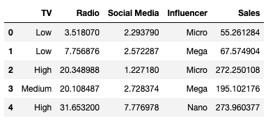
The features in the data are:

• TV: television promotion budget (Low, Medium, or High)
• Radio: radio promotion budget (in millions of dollars)
• Social Media: social media promotion budget (in millions of dollars)
• Influencer: type of influencer the promotion collaborated with (Mega, Macro, Nano or Micro)
• Sales: total of sales (in millions of dollars)

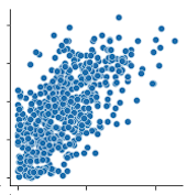
A pair plot is shown below:

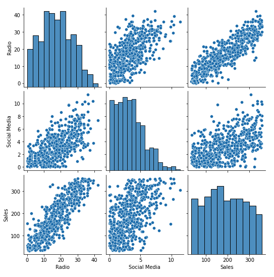
From the plot, we can see that both Social Media and Radio are positively correlated with Sales. If only one were to be selected, Radio appears to be a stronger indicator than Social Media, as the points cluster more closely around the fitted line. Thus, either Radio alone or the combination of Radio and Social Media could plausibly be selected as independent variables.

The mean Sales for each category in TV and for each category in Influencer are:

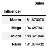
There is substantial variation in mean sales across the categories of TV, while mean sales vary very little across Influencer categories. The result indicates that TV should be retained as an independent variable, while Influencer can reasonably be discarded.

As the ols() function in Python doesn’t accept  variable names containing spaces, we rename Social Media to Social_Media.

Based on the analysis above, our task is to choose between the following two models:

1. Sales ~ C(TV) + Radio + Social_Media
2. Sales ~ C(TV) + Radio

2. The Pitfall in the Use of Variance Inflation Factor (VIF)

For the succeeding sections, assume we have imported the following libraries in Python:

import pandas as pd
import statsmodels.api as sm
from patsy import dmatrices
from statsmodels.stats.outliers_influence import variance_inflation_factor

The exemplar then fits the OLS model of Sales ~ C(TV) + Radio, tests the model assumptions of linearity, residual normality, and homoscedasticity, which are methodologically sound applications.

However, the method by which the exemplar checks the no multicollinearity assumption is worth reexamining.

The exemplar runs the following code to compute the VIF values for Radio and Social_Media:

x = data[['Radio','Social_Media']]
vif = [variance_inflation_factor(x.values, i) for i in range(x.shape[1])]
df_vif = pd.DataFrame(vif, index = x.columns, columns = ['VIF'])
df_vif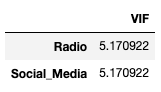

The exemplar concludes that the VIF when both Radio and Social_Media are included in the model is 5.17 for each variable, indicating high multicollinearity.

By revisiting the method, we find that the exemplar’s application leads quickly to the conclusion that Social_Media should be excluded due to multicollinearity, without comparing alternative model specifications.

To understand why this matters, it is useful to briefly revisit what VIF measures. The variance inflation factor (VIF) is one of the most widely used diagnostics for multicollinearity, largely due to its simplicity and broad applicability. It quantifies how much the variance (and thus uncertainty) of a regression coefficient increases due to multicollinearity among predictors, relative to a model in which the predictors are independent. Higher VIF values indicate less stable coefficient estimates that are more sensitive to small changes in the data.

For a given predictor $X_j$ ​, the VIF is defined as

where $R_j^2$​ is obtained by regressing $X_j​$ on all other predictors in the model.

In practice, VIF values are commonly interpreted using the following suggestive (rather than definitive) thresholds: a VIF of 1 indicates no multicollinearity; values between 1 and 5 suggest mild and typically acceptable multicollinearity; values between 5 and 10 indicate moderate and potentially concerning multicollinearity; and values greater than 10 are often taken as evidence of severe multicollinearity.

A more robust application in this case consists of the following steps:

1. Computing VIF with an intercept
2. Using the same design matrix as the regression model, including the categorical variable TV
3. Evaluating alternative model specifications to assess the marginal contribution  of Social_Media

Let’s begin with the reasoning behind step 1: Add intercept to calculate VIF. VIF measures how well one column can be explained by the other columns in the design matrix. When we omit the constant (intercept), we force every auxiliary regression to go through the origin. That changes the $R^2$. What the statsmodels internally run is $\text{Radio} = \beta \cdot \text{Social\_Media}$ (no intercept), whereas we actually want the model to be $\text{Radio} = \beta_0 + \beta \cdot \text{Social\_Media}$. That’s why we need to update the code to include the intercept:

x = data[['Radio','Social_Media']]
x = sm.add_constant(x)
vif = [variance_inflation_factor(x.values, i) for i in range(x.shape[1])]
df_vif = pd.DataFrame(vif, index = x.columns, columns = ['VIF'])
df_vif

This gives us the result:

The result aligns more closely with the correct analytical interpretation than the previous one.

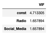
However, this is not sufficient on its own. By definition, VIF should be computed using the same design matrix as the regression model including the intercept, because multicollinearity is a group-level phenomenon. Multicollinearity is not about any single pair of variables. It is about near-linear dependence among a set of predictors. As we’ve decided to include categorical variable TV into the model, we should use the same design matrix in the code. A modified code could be:

y, X = dmatrices('Sales ~ C(TV) + Radio + Social_Media',data,return_type='dataframe')
vif = [variance_inflation_factor(X.values, i) for i in range(X.shape[1])]
df_vif = pd.DataFrame(vif, index = X.columns, columns = ['VIF'])
df_vif

patsy’s dmatrices adds the intercept. It also returns the same encoded TV dummies aligned with statsmodels, because statsmodels internally uses patsy. The full design matrix of the right-hand side of the formula is saved in X. The code returns the result:

Once VIF is computed on the full regression design matrix, VIF for Radio is 3.46, for Social_Media 1.66, and for TV dummies below common concern threshold (we should always ignore intercept’s VIF in our interpretation), suggesting no problematic multicollinearity.

To determine whether Social_Media should be excluded as an independent variable, we compare the model summaries from two specifications:

A. Model without Social_Media:

B. Model with Social_Media:

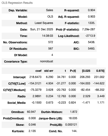
We can see that Model A exhibits strong overall fit, with all coefficients statistically significant, an adjusted $R^2$ of 0.904, and a highly significant F-statistic. Model B doesn’t seem to be an improvement from A, with Social_Media’s p value of 0.824, and Adjusted $R^2$ of 0.903 which is slightly worse than Model A’s. Per model results, we can now safely drop Social_Media.

Based on the analysis above, unlike the exemplar’s conclusion, we are not dropping Social_Media because of multicollinearity. We are dropping it because it adds no marginal explanatory power once Radio and TV are already in the model. The lack of significance is due to redundancy, not problematic multicollinearity.

Through this case study, working on these steps helped clarify several common misconceptions and led to three key principles for interpreting VIF, which are discussed in the following sections.

3. Principle 1: High correlation does not automatically imply multicollinearity

Multicollinearity refers to a situation in which one or more predictors in a regression model can be well approximated by a linear combination of the others.

For now, consider the simplified case of two predictors.

Examining standard (suggestive rather than definitive) VIF interpretation guidelines, one may notice that the threshold for diagnosing multicollinearity in the two-predictor case appears unusually strict. When only two predictors are present, the correlation coefficient must exceed approximately 0.9 before VIF reaches a value of 5, a value that is commonly used to flag potential multicollinearity. This is because, with two predictors, the squared correlation coefficient is equivalent to the $R^2$ obtained by regressing one predictor on the other. Substituting this into the VIF formula, $\text{VIF} = \frac{1}{1 – r^2}$, yields a value of approximately 5 when r=0.9.

By contrast, although there is no universal cutoff for “high” correlation, values above 0.6 are often considered strong and are visually apparent in scatter plots. However, when r=0.6, the corresponding VIF is only about 1.56, which is well below commonly used thresholds for concern.

Following is a scatter plot of two variables with a correlation coefficient of 0.63, corresponding to a VIF of approximately 1.66:

The key intuition linking these observations is that even at moderately high correlation levels, a substantial portion of variation remains unexplained. For example, when r=0.6, roughly 64% of the variance is unexplained, and even when r=0.8, about 36% remains unexplained. In such cases, an additional predictor can still provide meaningful marginal explanatory power, which is why high correlation alone does not imply problematic multicollinearity under a rigorous definition.

Notably, as the correlation coefficient approaches 1, VIF increases rapidly and nonlinearly. While the two-predictor case requires extremely high correlation to trigger concern, the presence of additional predictors changes this dynamic. With multiple predictors, even moderate pairwise correlations can inflate VIF. For this reason, all predictors should be included when computing VIF to ensure that the diagnostic reflects the full regression design.

4. Principle 2: Multicollinearity does not imply high pairwise correlation

Correlation is fundamentally a bivariate concept. When discussing correlation among multiple variables, we are typically referring to pairwise correlations between variable pairs.

It is possible to construct a case where pairwise correlations are low or even zero, yet multicollinearity is present.

Consider the constructed example $X_5 = X_1 + X_2 + X_3 + X_4 +\epsilon$, where $X_1$, $X_2$, $X_3$, and $X_4$ are mutually uncorrelated, and $\epsilon$ is a noise term independent of the other predictors. By construction, pairwise correlations between predictors can be small, including those involving $X_5$​. Intuitively, the noise term increases the overall variability of $X_5$​ without increasing its shared variation with any single predictor, allowing pairwise correlations to remain small. However, when considered jointly, $X_5$​ can still be well explained by a linear combination of $X_1$,$X_2$,$X_3$ and $X_4$, resulting in strong multicollinearity in a regression model of the form $Y = aX_1 + bX_2 + cX_3 + dX_4 + eX_5 + intercept$.

This example illustrates that multicollinearity does not imply high pairwise correlation. Consequently, multicollinearity should be assessed using the full regression model, rather than inferred from pairwise correlations alone.

5. Principle 3: A higher VIF does not imply that a variable should be dropped

This case study clarifies a common misunderstanding in the interpretation of VIF. VIF values should not be compared mechanically across predictors to determine which variable to remove from a regression model.

Multicollinearity is a group-level issue among predictors: removing any one of the collinear variables can restore model stability, and the final choice should be based on each variable’s marginal contribution to explaining the response. In other words, VIF diagnoses group instability, not variable importance.

The marketing case discussed above illustrates this clearly. Although the VIF for Radio (3.46) is higher than that for Social_Media (1.66), Social_Media is the variable that is removed from the model. This shows that variable selection should be guided by marginal explanatory power rather than by relative VIF values alone.

In predictive modeling contexts, where the primary goal is generalization rather than coefficient interpretability, multicollinearity is often addressed through regularization techniques—such as Ridge, Lasso, and Elastic Net—rather than explicit variable removal. However, since the focus of this discussion is the interpretation and application of VIF, these models will not be explored in detail here.

6. Conclusion

This case study illustrates that multicollinearity is fundamentally a group-level phenomenon and cannot be reliably inferred from pairwise correlations alone. VIF serves as a diagnostic tool for assessing instability among predictors within a specified regression model, which is why it must be computed using the full design matrix, including the intercept. However, diagnosing multicollinearity is only one step in model building. Decisions about whether to retain or remove predictors should ultimately be guided by their marginal contribution to explaining the response, rather than by VIF values in isolation. Used in this way, VIF supports sound modeling decisions rather than replacing them.